Please see me my other Excel articles.

Leveraging Z-Score to Understand Data Dispersion

In my Standard Deviation article I demonstrated how to use the squared variance to show the average distance each data point resides from the mean.

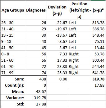
While variance and standard deviation illustrate data dispersion from the mean in terms of their precise location in relation to the mean, Z-Score provides another measurement of dispersion from the mean, but using the standard deviations to provide a more high-level measurement.

Recall from my Distributions: The empirical rule article (link), in a normally-shaped distributed, most data points fall within three standard deviations from the mean.

Referencing standard deviations in this manner provides an easy-to-use reference in understanding variance in relation to the mean instead of actual values.

Similarly, z-scores use standard deviations to understand data points’ variance in relation to the mean.

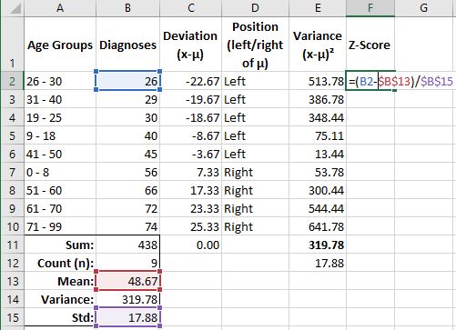
With my new Z-Score column, I now have a value which tells how many standard deviations from the mean (negative-left, positive-right) each value resides from the mean.

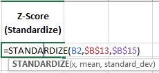
Also, Excel provides the Standardize() function to determine z-scores.

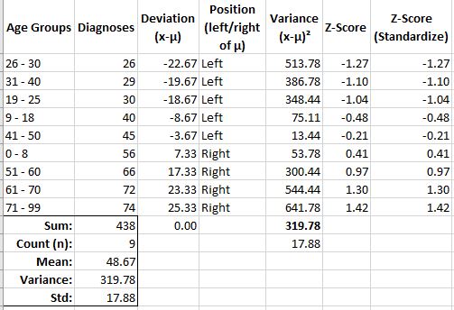
For example, the last z-score of 1.42 is for the age group of 71-99. This tells me this age group’s diagnoses of 74 falls almost 1.5 standard deviations above (positive – right of) the mean.

Also, the z-score may be used with a z-table to determine its value in relation to all other values.

Z-table

Continuing with the z-score for the 71-99 age group (1.42), I can use the following Z-table to determine data points under this value.
https://www.statisticshowto.datasciencecentral.com/tables/z-table/

Beginning with the left Z column and finding 1.4, then going two columns to the right for the .02 (1.4 + .02 = 1.42), I get a value of .4222, or 42%.
Since this z-table tells me “Use these values to find the area between z=0 and any positive value.,” this value tells me beginning with z=0 (the mean), 42% of all other data points to the right of the mean (positive z-scores) fall under the diagnoses of 74. Since the right area of this distribution is only half the distribution (the other half has negative values), I can add 50% to represent that half to 42%, to arrive at a total of 92% of all values fall below (to the left of) this diagnosis in the distribution.
To determine how much data falls above this value, I simply subtract 1 from this value (1 – 92%) to arrive at 8%. Remember from my Distributions: The empirical rule article (link) approximately .03% of data falls outside the standard three standard deviations. Therefore, the amount of data above the diagnosis of 74 for the age group 71-99 is actually 8% – .03% = 7.97%.

This means the highest number of diagnosis (74) for the age group 71-99 resides above 92% all other diagnosis in the distribution with less than 8% residing above it.