Creating a list lookup.

Many Excel spreadsheets contain data spread across many different worksheets and in collaboratively work environments, worksheets are shared among coworkers.
The result of this data separation is that sometimes a scenarios arises when critical data is needed but unavailable by the current spreadsheet.
To overcome this limitation, I will use the Excel VLookup formula to compare a key field on one worksheet against another key value in a separate worksheet.
First, I’ll begin with simple Sales worksheet containing three orders (1-3).
Notice the column “Sale Associate” which references another worksheet.

The second worksheet I have is the actual lookup used to retrieve the names of Sales Associates.
Ensure this worksheet’s key column (the values used to as a reference by the first worksheet) is the first column.
First, I’ll insert a new formula by searching for VLookup.

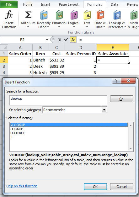Once found, I’m prompted by three required and one optional fields.

For the first argument, I’ll specify I want the key lookup fields to be the “Sales Person ID” value (not column).
Next, I’ll click inside the second argument and select the “Sales Associates” worksheet tab and highlight all available cell values excluding column headers.

Finally, for the third argument indicating which column’s data to retrieve, I’ll enter ‘2’ for the second “Name” column in the worksheet.

Upon pressing [ENTER] the first sales name is listed in the first worksheet by pulling it from the second worksheet.

To implement the lookup on the other Sales Associate values, I’ll simply drag/copy the cell’s formula to the other two cells.