Consolidating data into one Excel worksheet.

This post describes how to merge data in an Excel workbook containing worksheets with data where each worksheet has differing number of columns and rows.
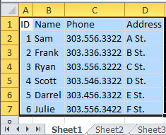
I will use a spreadsheet which contains three tabs/worksheets with the following columns.

Sheet1 will be the first source worksheet used to import data.

Sheet2 will be the first source worksheet used to import data.Sheet3 will serve as the target for the data import from Sheets 1 and 2.

Steps

Use the following steps to merge data from multiple data sheets into a single data sheet:

1. Define Worksheet Names.
2. Configure the data import process.

1) Define Worksheet Names
In this step you will prepare the source Worksheets for use in the import process by assigning intuitive names for them for use in the import process.

a) Select the first source tab and highlight all data to be imported.

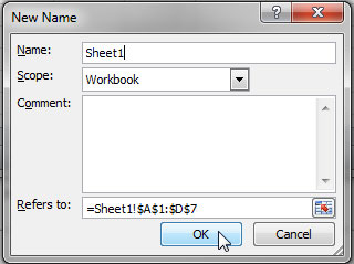
b) Execute the Define Name wizard: Top Menu -> Formulas -> Define Name -> Define Name

c) Assign an intuitive name and optional Comment for the current tab that you will remember in a future step, OK.

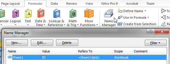
Should you make a mistake or later wish to change the name you assigned, use the Name Manager.

Repeat this step for other source Worksheet(s).

2) Configure the data import process.

a) Select the target Worksheet where you are expecting to import data, and place the cursor in the top-left cell.

b) Execute the data import process.

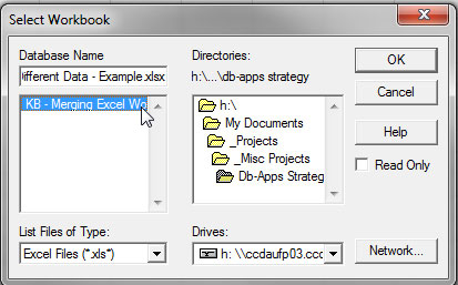
d) For Databases, choose Excel Files*, OK.

(you will see this window)

e) Navigate to where your Spreadsheet/Workbook resides, select it, then OK.

f) Add both sheets into the right box, Next.
(you want all columns)

You will receive a warning that you must “join the tables manually”, OK.

(the Microsoft Query windows opens)

g) Now you simply decide which column is the link between the two – this will be the column with identical values. It is highly recommended you use numeric values for this “key.”
You may elect to use the many query button to remove certain columns from the output, affect a sort order, etc.

In this example, I dragged ID from the left unto the right ID.

Once you “link” the two sheets, you will see a preview of which data satisifies the “relationship” between both sheets. In this case, the final result will be quite small since there were no ID=3 records.

h) Once you are satisfied with your final data set, send the data back into your third tab.

i) You will prompted to confirm where you want the data, OK.

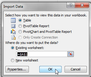
Final Data set

I now have my final data set, complete with filters and basic styling.

Note: If the final data set seems too small, ensure in both source tabs no duplicates exist.