Using Excel to View Cubes and Configure Pivot Table Reports

Similar to my article SSAS BIDS Cube Browser, Microsoft provides another tool for any end user to view a cube’s measures and dimensions to configure highly analytical reports.

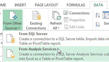
First, use the wizard under the Data tab to configure an connection to your cube.

In the first window, choose your server and authentication.

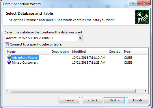
In the final window, save your connection information and click Finish.

When prompted, select to create a Pivot table within the existing spreadsheet.

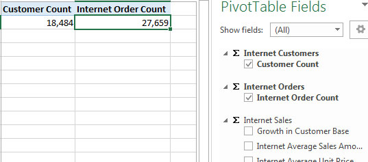
You will see a workspace to configure your Pivot tale view of the cube.

I will select the first two measure which automatically display their values in my table area.

To more easily compare the difference between the number of customers I have and their number of order, I will move the values from Columns to Rows to see them displayed above/below each other.

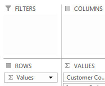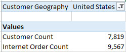
Next, I would like to see those numbers by customer geography so I will add a Customer Geography dimension and move it from the ROWS area to become a filter.

Now I may use the Customers filter to only see counts from USA customers.